Temporally coherent disparity maps using CRFs with fast 4D filtering

Abstract

State-of-the-art methods for disparity estimation achieve good results for single stereo frames, but temporal coherence in stereo videos is often neglected. In this paper, we present a method to compute temporally coherent disparity maps. We define an energy over whole stereo sequences and optimize their conditional random field (CRF) distributions using the mean-field approximation. In addition, we introduce novel terms for smoothness and consistency between the left and right views. We perform CRF optimization by fast, iterative spatio-temporal filtering with linear complexity in the total number of pixels. We propose two CRF optimization techniques, using parallel and sequential updates, and compare them in detail. While parallel updates are not guaranteed to converge, we show that, in practice with appropriate initialization, they provide the same quality as sequential updates and they also lead to faster implementations. Finally, we demonstrate that the results of our approach rank among the state of the art while having significantly less flickering artifacts in stereo sequences.

1 Introduction

While some disparity estimation methods leverage information over several frames of stereo video sequences, most do not attempt to produce temporally coherent disparity maps. In applications like video production for 3D displays, however, temporally coherent disparity maps are crucial. While human observers are more forgiving about incorrect disparities, they easily notice flickering artifacts due to temporally incoherent disparity maps.

We address these challenges by proposing a technique that produces temporally coherent disparity maps over stereo videos. We formulate an energy minimization problem consisting of unary, smoothness, and consistency terms, which we solve using the mean-field approximation of a densely connected conditional random field (CRF). We propose two efficient filtering techniques to solve the mean-field approximation, using parallel and sequential updates. Both have linear complexity in terms of the number of pixels in the input. Parallel updates allow us to process all pixels in a stereo sequence independently, enabling fast GPU implementations. In contrast to sequential updates, parallel updates are not guaranteed to converge. We provide a detailed comparison between both techniques and show that, with proper initialization, parallel updates obtain the same quality of results. Hence, they are preferable in practice.

In summary, our contributions are (1) a new smoothness term that leverages both the left and right images to distinguish between image edges due to disparity discontinuities, and edges due to surface texture; (2) a novel consistency term to obtain a joint left-and-right disparity estimation problem; (3) a temporal smoothness term to achieve temporally coherent disparity maps over stereo video sequences; (4) a comparison of efficient CRF optimization techniques based on parallel and sequential updates.

Figure 1 shows a comparison of disparity maps from three techniques that support spatio-temporal disparity estimation, including TDCBG [23], PRSM [28], and our method. We used the maximum temporal support for each method, which is eight consecutive frames for TDCBG, three frames for PRSM, and 21 frames for our approach. On the right side of Fig. 1, we show the average disparity flicker index in this sequence. The flicker index is a quantitative measurement of the temporal smoothness of a signal, and we compute it according to the IESNA standard [4]. Our algorithm and TDCBG [23] allow controlling temporal smoothness with a user-specified parameter σ _t . Our proposed algorithm achieves the lowest flicker index, can be computed in linear complexity in terms of image resolution and number of frames, and our GPU implementation requires only a few seconds per frame. Finally, our method ranks among the state of the art in the KITTI benchmark [9].

Fig. 1

Our optimization includes the temporal dimension to achieve temporally coherent disparity maps in linear time. Here, we compare disparity maps from TDCBG [23] using a temporal window of eight frames, PRSM [28] using three frames, and our method using 21 frames. We also indicate the computation time per frame for each method. On the right, we show the average disparity flicker index in this sequence. Our algorithm and TDCBG [23] allow controlling temporal smoothness using a temporal support parameter σ _t . Sequence courtesy of MEDIA LEADER Srl (www.medialeadersrl.com)

The rest of this paper is organized as follows: after discussing previous work in Section 2, we introduce our energy formulation that includes a novel consistency term and the temporal extension in Section 3. Next, in Section 4, we discuss energy minimization via the mean-field approximation and using an iterative algorithm with parallel updates. Parallel updates are not guaranteed to converge, however, and we develop an efficient sequential approach in Section 5 that does not suffer from this problem. Finally, we evaluate our approach using standard datasets in Section 6.

This paper is based on a conference publication [1]. Here, we describe the method in more detail and provide further analysis of the CRF inference scheme. We also develop a novel, efficient sequential approach that guarantees convergence unlike the previous parallel approaches. We evaluate the parallel and sequential techniques and conclude that, in practice with appropriate initialization, parallel updates lead to equivalent results but can be implemented more efficiently.

2 Related work

Disparity estimation is commonly defined as a discrete labeling problem. Aggregation-based methods [22] share the cost of each assignment with neighboring pixels to reduce noise. They are efficient but unable to reason about more complex assignment configurations. Optimization-based methods try to find the best assignment of disparities by minimizing an energy function. Semi-global matching (SGM) [12] is a fast and effective approach that enforces local smoothness over many directional scan-lines using dynamic programming. Methods such as wSGM [24] and i-SGM [11] modified the original SGM to improve performance. žbontar and Yann [32] used convolutional neural networks to define a new unary term for SGM that leads to significant quality improvements but incurs a high computational cost. While SGM is able to find a semi-global establishment of disparity labels, it is unable to capture the local structure due to the simple energy function.

On the other hand, filter-based mean-field approximation [17] supports very fast optimization over a fully connected CRF. Yu and Gallup [31] used this approach to obtain disparity maps. Vineet et al. [26] further extend the optimization to include higher order terms that incorporate information about objects to be used in the disparity estimation problem. Many methods use a multi-scale approach to increase robustness to local minima [33]. Zhang et al. [33] aggregate the cost between different scales such that the assignment is consistent in all scales. Vineet et al. [25] run the optimization on coarser scales to initialize finer ones. We use the SGM method to initialize our CRF-based optimization, which further incorporates other complex terms.

Some methods use several stereo frames and attempt to ensure temporal coherence. Slanted plane StereoFlow [30] uses two consecutive frames to improve results. The method computes an initial disparity map using SGM and then jointly optimizes for planar surfaces and local segments. This approach is tailored for applications such as autonomous vehicles with an ego-motion assumption. Vogel et al. [28] use consistency factors between the views that are defined as a data term in their optimization. Using a piecewise rigid model, their method includes consistencies in the temporal dimension that incorporates neighboring views. Unlike these methods, we do not enforce segmentation nor local planarity on our disparity maps. In addition, our method has linear complexity with respect to the number of frames, which allows us to compute the disparity maps of the whole sequence in a single optimization.

Disparity flicker artifacts have been previously addressed [21, 23]. Richardt et al. [23] assumed that the pixel’s disparity persist in time and aggregated the costs between temporally consecutive pixels. Min et al. [21] filtered noisy disparity maps between different frames. Similar to their work, we use a precomputed flow field and enforce temporal coherence along its vectors. In addition to end-to-end disparity error, we propose a quantitative measure to better evaluate the flicker artifacts in disparity sequences and compare with previous works.

3 Energy terms

In this section, we describe our energy terms that characterize the spatio-temporal disparity estimation problem. We assume that the stereo inputs are rectified such that the disparity is only in the horizontal direction, but our method is not limited to this setup. We define random variables ${x^{L}_{i}}$ for the disparity values of pixels i, where i determines the spatial location of the pixel, in the disparity field X ^L of the left image, and similarly ${x_{i}^{R}}$ in X ^R for the right image. Our joint energy function over X ^L and X ^R includes unary (per pixel), smoothness, and consistency terms. We omit the left and right superscripts unless necessary.

3.1 Unary term

We denote the cost of assigning disparity d to pixel i in the left image L by the unary term ${\phi _{u}^{L}}(x_{i} = d)$. We compute this term using a standard approach, which is based on edge differences and census transform distances similar to Yamaguchi et al. [30]. Specifically,

$$\begin{array}{*{20}l} &{\phi_{u}^{L}}(x_{i} = d) = \\ &\frac{1}{|N(i)|}\sum_{j \in N(i)} \left\{ |{S^{L}_{j}} - S^{R}_{j+d}| + \lambda_{cen} |H({T^{L}_{j}}, T^{R}_{j+d})| \right\}, \end{array} $$

(1)

where ${\phi _{u}^{L}}(x_{i} = d)$ is the unary cost of assigning disparity d to pixel i in the left image, S ^L and S ^R denote the response to the horizontal Sobel operator, H is the Hamming distance of the center-symmetric census transforms T ^L and T ^R introduced by Spangenberg et al. [24], and $\lambda _{\text {cen}} = \frac {1}{3}$ is a constant that controls the relative weight of the two terms. The cost for pixel i is averaged over its 8-connected neighbors j∈N(i). We compute the census transform in a 7×7 window on the blurred image using a 3×3 box filter. This will increase robustness against artifacts such as noise and aliasing. The census transform is a feature that represents the local arrangement of pixels in a neighborhood robust to brightness changes and noise by capturing if the brightness of a pixel is larger than the center pixel of that neighborhood. Since this transformation looses some textural information, adding the edge difference measure helps to better identify the matching pixels in the other view.

3.2 Disparity-dependent smoothness term

The goal of the smoothness term is to encourage pairs of pixels that are close in some sense (defined more precisely below) to get similar disparity assignments. We define the smoothness term ${\phi _{s}^{L}}(x_{i}=d_{i}, x_{j}=d_{j})$ for a pair of assignments x _i =d _i and x _j =d _j in the left image as a function of both the pixel locations i,j and the disparity assignments d _i ,d _j (similarly for the right image). We express this term as a sum of weights W ^L(P) over all paths P that connect the points 〈i,d _i 〉 and 〈j,d _j 〉 in the joint pixel-disparity space,

$${\phi_{s}^{L}}(x_{i}=d_{i}, x_{j}=d_{j}) = -\left(\sum_{P \in \mathcal{P}(i,d_{i},j,d_{j})} W^{L}(P)\right), $$

where $\mathcal {P}(i,d_{i},j,d_{j})$ is the set of all paths between 〈i,d _i 〉 and 〈j,d _j 〉 in the joint space of pixel locations and disparity hypotheses and each path P={〈k,d〉} is a sequence of (4-connected) pixels k paired with a disparity hypothesis d.

We define the weight kernel W based on three length functions of the path: its length l _s (P) in the image, its length l _d (P) in the disparity label space, and a length δ ^L (discussed below) that takes into account potential disparity discontinuities along the path. Specifically, the weight kernel is

$$ W^{L}(P) = \exp \left\{ {-\left|\left| \frac{\delta^{L}(P)}{\sigma_{r}} + \frac{l_{s}(P)}{\sigma_{s}} + \frac{l_{d}(P)}{\sigma_{d}} \right|\right|_{2}^{2}} \right\}, $$

(2)

where σ _r ,σ _s , and σ _d control the kernel support for the three length terms. Applying a Gaussian weight to the sum of the three distances ensures that W ^L(P) decreases when the two pixels are separated by a large distance and it increases when they are close. Because we sum the negative weights W ^L(P) over all paths, the smoothness energy (cost) decreases by the weight of each path and each short path further reduces the energy. In contrast, Hosni et al. [13] used only the path with the minimum distance. A single path, however, is more sensitive to noise. Summing up the weights from all paths not only includes the weight from the shortest path but also increases robustness to noise. Additionally, including all paths favors arrangements where assignments are connected by many long paths in contrast to assignments with few short paths. This choice of weight will later allow us to efficiently compute the smoothness energy.

The key ingredient in the definition of W ^L(P) is the length δ ^L(P), which we design to become large when the path crosses depth discontinuities. Since depth discontinuities are not known a priori, either boundaries in superpixel segmentation [28, 30] or image edges (pixel-wise differences) [5, 17, 19, 22, 25, 32–34] are conventionally used in their place. Many image edges, however, represent surface texture, not depth discontinuities; hence, these approaches may lead to ineffective smoothness energies. Crucially, we consider color information from both (left and right) views to compute the path length δ ^L(P) such that it depends on the disparities along the path P. For each disparity on the path, we compute a pixel-wise difference of the two views where one is shifted by that disparity. At pixels where the disparity happens to be the correct one, this will cancel image edges due to surface textures, indicating that these edges are not disparity discontinuities. If the disparity is wrong, image edges typically do not cancel. We use this intuition to define a disparity discontinuity indicator for pixel k and disparity d as min(|L _k −R _k+d |,|L _k −L _k−1|), where L and R denote the left and right color images, and pixels k−1 and k+d are horizontally offset from pixel k. Taking the minimum makes sure we do not introduce any spurious discontinuities. The path length δ ^L(P) is now simply the sum of these disparity discontinuity indicators along the path,

$$\delta^{L}(P) = \sum_{\left\langle k, d\right\rangle \in P} \min(|L_{k} - R_{k+d}|, |L_{k} - L_{k-1}|). $$

This distance will be small if the pixel colors along the path have correspondences in the other image under their disparities, even if the image itself has large color dissimilarities along that path.

We visualize our approach in Fig. 2. We show slices of the joint pixel-disparity space (d,i), where disparities d are along the horizontal axis, and the vertical axis corresponds to one vertical column of pixels i. The data is from a continuous, slanted surface patch that is highly textured (ground region in Fig. 8, top left). Figure 2 a shows conventional disparity discontinuity indicators given by pixel differences |L _i −L _i−1|, and Fig. 2 d is our proposed indicators min(|L _i −L _i−1|,|L _i −R _i+d |). Figure 2 a, d shows the ground truth disparities in red and some estimated disparities consisting of fronto-parallel segments in green. In Fig. 2 b, c, e, f, we visualize the smoothness energy for the red and green disparity assignments using the conventional and our approach. That is, each point (d,i) in these figures shows the sum $\sum _{j} {\phi _{s}^{L}}(x_{i}=d, x_{j} = \Delta _{j})$ where the Δ contains either the ground truth (red) or estimated (green) disparities. We also indicate the total smoothness energy $\sum _{i,j} {\phi _{s}^{L}}(x_{i}=\Delta _{i}, x_{j} = \Delta _{j})$. This shows that in the conventional approach some pixels have high smoothness energies even with the ground truth disparity assignment, and the total smoothness energy of the piecewise fronto-parallel disparities (green, Fig. 2 c) is actually lower than the ground truth (red, Fig. 2 b) here. With our approach, we obtain low smoothness energies at all pixels, and the ground truth (red, Fig. 2 e) has lower energy than the piecewise fronto-parallel assignments (green, Fig. 2 f).

Fig. 2

Visualization of the smoothness energy in the joint pixel-disparity space (pixels i on vertical axis, disparities d on horizontal axis). The top row shows the conventional approach, and the bottom row is our technique, where a is the conventional disparity discontinuity indicator, and d our proposed one. The red line in the left and middle columns indicates the ground truth disparities, and the green line in the left and right columns is a piecewise fronto-parallel disparity assignment. In the conventional approach, the piecewise fronto-parallel disparities incorrectly have a lower smoothness energy (−0.6 in c) than the ground truth (−0.4 in b). Our technique correctly leads to a lower energy for the ground truth (−1.9 in e) compared to the fronto-parallel disparities (−1.8 in f)

3.3 Higher order local consistency term

Each disparity assignment indicates that the corresponding pixel appears with a shift (disparity) in the other image; therefore, we expect that the disparity in the other view would agree with this assignment. We design the consistency energy to be low if the disparity assignments in two corresponding pixels in the left and right images agree. As a key idea, we compute this term over pixel neighborhoods, instead of individual pixels, to be more robust to per-pixel errors. We first introduce a binary consistency factor $\nu = [|{x^{L}_{j}} - x^{R}_{j+{x^{L}_{j}}}| \leq 1 ]$, which is one when two corresponding pixels ${x^{L}_{j}}$ and $x^{R}_{j+{x^{L}_{j}}}$ (according to the disparity assignment in the left image) agree on their disparities up to a threshold of one disparity level, and zero otherwise. We allow for a difference of one disparity level to compensate for sub-pixel disparities and self-occlusions. We now define the consistency energy as

$${\phi^{L}_{c}}({x_{i}^{L}} = d_{i}, {x_{j}^{L}} = d_{j}) = -\left(\sum_{P \in \mathcal{P}(i,d_{i},j,d_{j})} W^{L}(P)\right) \nu, $$

where we sum over all paths between joint pixel-disparity assignments ${x_{i}^{L}}$ and ${x_{j}^{L}}$ and use the same path weight W ^L(P) as for the smoothness term. Note that although this term is defined over pairs of disparity variables in one view, it implicitly involves a third disparity variable from the other view via the disparity compatibility function ν. Intuitively, given an assignment ${x_{i}^{L}}$, our consistency energy is low if many assignments ${x_{j}^{L}}$ that are close to ${x_{i}^{L}}$ in the left image have consistent assignments $x^{R}_{j+{x^{L}_{j}}}$ in the right image. Since we cannot confirm consistency in the case of occlusions, we ignore them here and treat them later when finalizing the disparity map.

3.4 Temporal extension

A main advantage of our filter-based CRF optimization (Section 4) is that we can easily extend it to the temporal domain and simultaneously optimize disparity assignments over all frames of a stereo video sequence. By extending the smoothness and consistency terms to the temporal dimension, we will obtain temporally coherent disparity maps that reduce flickering artifacts. We define the smoothness and consistency energies (ϕ _c ,ϕ _s ) as before but now with weight kernels W over paths in the joint spatio-temporal and disparity domain,

$$W^{L}(P) = \exp \left\{ {-\left|\left| \frac{\delta^{L}(P)}{\sigma_{r}} + \frac{l_{s}(P)}{\sigma_{s}} + \frac{l_{t}(P)}{\sigma_{t}} + \frac{l_{d}(P)}{\sigma_{d}} \right|\right|_{2}^{2}} \right\}, $$

where l _t (P) is the length of the path in time and σ _t determines the kernel width along time. Our assumption here is that the disparities persist over a short time defined by σ _t . As a key idea, we define the temporal dimension by following flow vectors of a precomputed flow field over the video sequence. Specifically, we use the flow by Lang et al. [18] and refer the reader to their paper for more details.

4 Energy minimization

Here, we describe our fast spatio-temporal energy minimization based on the mean-field approximation and using parallel updates of the mean field. In addition, we discuss initialization and post processing, followed by a description of our GPU implementation.

4.1 Mean-field approximation

We define the global energy function E as a sum of the unary, smoothness, and consistency terms, all evaluated on both the left and right images,

$$\begin{aligned} E(X^{L}, X^{R}|L, R) = & \sum_{i}\left\{{\phi_{u}^{L}}(x_{i}) + {\phi_{u}^{R}}(x_{i})\right\} \\ & + \lambda \sum_{i,j}\left\{{\phi_{s}^{L}}(x_{i}, x_{j}) + {\phi_{s}^{R}}(x_{i}, x_{j})\right\} \\ & + \gamma \sum_{i,j} \left\{{\phi^{L}_{c}}(x_{i}, x_{j}) + {\phi^{R}_{c}}(x_{i}, x_{j})\right\}, \end{aligned} $$

with parameters λ and γ to control the influence of the smoothness and consistency terms relative to the unary term.

We can relate this energy to the probability distribution of the disparity, which takes the form of a conditional random field (CRF),

$${\text{Prob}}(X^{L}, X^{R}|L, R) = \frac{1}{Z(L, R)}\exp(-E(X^{L}, X^{R}|L, R)), $$

where $Z(L, R) = \sum _{X^{L}, X^{R}}\exp {(-E(X^{L}, X^{R}|L,R)}$ is a partition function that normalizes the probabilities to add to one.

We minimize the energy function by following the filter-based mean-field approximation [17]. The mean-field approximation estimates the distribution Prob(X ^L,X ^R) with a much simpler distribution Q(X ^L,X ^R) in which the variables are marginally independent, that is, $Q(X^{L}, X^{R})=\prod _{i}{{Q^{L}_{i}}({x^{L}_{i}}){Q^{R}_{i}}({x^{R}_{i}})}$, where ${Q^{L}_{i}}({x^{L}_{i}})$ and ${Q^{R}_{i}}({x^{R}_{i}})$ are the marginal distributions of all variables (pixels) in the left and right images. Using this assumption, one can iteratively update probabilities for each variable assignment independently by computing the expected value of the energy conditioned to that assignment. For the disparity distribution in the left image, this is

$$ \begin{aligned} &{Q_{i}^{L}}(d) = \frac{1}{Z_{i}} \exp \left\{{\vphantom{\sum_{j}}}-{\phi_{u}^{L}}(x_{i}) - \right.\\ &\left.\sum_{j} \left(\lambda \mathbf{E}[{\phi_{s}^{L}}(x_{i}, x_{j}) | x_{i}=d] + \gamma \mathbf{E}[{\phi^{L}_{c}}(x_{i}, x_{j}) | x_{i}=d] \right) \right\}, \end{aligned} $$

(3)

where Z _i is again the partition function that is used to normalize the distribution over the variable x _i . The summation over j accumulates the expected values E, conditioned to x _i =d, over all energy terms that include the variable x _i . The expected value for each smoothness term, conditioned to x _i =d, is

$$\begin{array}{*{20}l} \mathbf{E}[{\phi^{L}_{s}}(x_{i}, x_{j}) | x_{i}=d] = \sum_{l} {\phi^{L}_{s}}(x_{i}=d, x_{j}=l) {Q_{j}^{L}}(l), \end{array} $$

(4)

and for the consistency term it is

$$\begin{array}{*{20}l} &\mathbf{E}[{\phi^{L}_{c}}(x_{i}, x_{j}) | x_{i}=d] = \\ &\sum_{l} \sum_{k=l-1}^{l+1} {\phi^{L}_{c}}(x_{i}=d, x_{j}=l) {Q_{j}^{L}}(l) Q_{j+l}^{R}(k). \end{array} $$

(5)

Here, the sum over k∈{l−1,l,l+1} corresponds to the compatibility function ν in Section 3.3. Although the consistency term ϕ _c is defined over three independent random variables, the expected value here is conditioned on the assignment of disparity d to pixel i; hence, the conditional expected energy only depends on the probabilities of the two remaining variables ${Q_{j}^{L}}$ and $Q_{j+l}^{R}$.

4.2 Filter-based parallel update iteration

Algorithm 1 minimizes our energy by iteratively updating the mean-field distributions by computing Eq. 3. The first iteration of the algorithm updates the disparity distribution of the left image (Q ^L). In subsequent iterations, we switch between updating the disparity maps of the left and right images (line 5) to avoid oscillations between them. The notation implies that the operations are applied to all variables i and values d in parallel. The first two lines in the loop compute the expected values (Eqs. 4 and 5) and the summation over all pixels j in Eq. 3. First (line 1), we compute intermediate values $\tilde {Q}_{i}$ that store the contributions that each pixel will make to the conditional expected energies of the smoothness and consistency terms of all other pixels. Next (line 2), at each pixel, we simultaneously compute the expected values (summation over l) and accumulate the contributions from all the other pixels (summation over j) using a single, fast filtering operation over the intermediate values $\tilde {Q}_{i}$. We provide some more details about the filter implementation below. A single filtering step is possible since we have the same weights W defined in ϕ _s and ϕ _c . In line 3, the disparity potential is computed by adding the unary term, exponentiating, and normalizing to a distribution in line 4, which completes computation of Eq. 3. Finally, the iteration ends by switching the target distribution (line 5).

A key element of our algorithm is that we compute the path weights W efficiently using the domain transform filter [7], which allows us to evaluate each filtering operation (line 2 of Algorithm 1) in constant time. We use interpolated convolution by iteratively applying a moving sum (box filter) in the transformed domain. The joint image and disparity space leads to 3D filtering, and our temporal extension to 4D filtering over two spatial, the temporal, and the disparity dimensions. In the temporal dimension, we filter along the precomputed flow vectors similar as Lang et al. [18]. We obtained our best results by iterating over passes along spatio-temporal directions and filter in the disparity domain at the end. We refer to the original publication [7] for more details about the domain transform filter.

4.3 Initialization

For initializing Algorithm 1, we leverage semi-global matching (SGM) [12] with penalties P ₁=4,P ₂=64 in four directions. Instead of the MAP results of SGM, we rather use the obtained (min-marginal) energies to initialize our distribution Q _i (d). For a better initialization, we run the first two iterations of the optimization using a large kernel support (σ _s =7,σ _r =100,σ _d =2).

4.4 Final disparity map

We compute final disparities by finding the one with the minimum energy − log(Q _i (d)) from Algorithm 1. For accuracy below the level of the disparity discretization, we fit a quadratic to the three disparity costs centered at the minimum. We remove spikes by applying a 5×5 median filter. We fill occluded regions by checking for left-right consistency to find pixels with disparity differences higher than a threshold and replacing disparities marked as occluded with the last non-occluded disparity in the left direction for the left view (similarly for the right view).

4.5 Implementation

The CPU version of the proposed pipeline supports 256 or more disparity hypotheses. We also implemented a GPU version for the whole pipeline that takes advantage of parallelism in the optimization at the pixel level. We ran our experiments on an Nvidia Titan Black graphics card with 6-GB memory on board. We allocate memory for a batch of left and right images, including the disparity hypothesis layers requiring 2×Width×Height×Frames×Disparities floating point values. Because of the limited GPU memory, we are currently restricted to batches of 14 frames at a resolution of 960×540 and 32 disparity layers. Note that we evaluate the unary term at a finer discretization of disparity steps, typically at one pixel steps. We then store the minimum for each of the 32 layers. At the end of the optimization, the disparity is computed and finalized as described above, and by fitting the quadratic to the 32 layers, we achieve finer levels of disparity. After the disparities of a batch of frames are computed, we move forward by seven frames and compute the disparities for the next batch. We finally interpolate the disparity values of the overlapping frames in consecutive batches for smoother transitions.

5 Convergence analysis

Our proposed Algorithm 1 in Section 3 and other filter-based mean-field approximation methods [17, 26] update the random variables in the mean-field in parallel. While parallel updates lead to very fast implementations, they are not guaranteed to converge at all. The goal of this section is to answer two questions: First, how good are results obtained using parallel updates of the mean-field compared to sequential updates, which are guaranteed to converge to a fixed point? Second, how well can the mean-field approximate our energy functional compared to methods that do not make the same assumption? To answer the first question, we develop an efficient method that applies mean-field inference with guaranteed convergence using sequential updates and we compare its results with the parallel implementation’s. Second, we compare our approach with the minimized energy of Graph Cuts [2], which does not rely on the mean-field approximation.

To explain the sequential algorithm more clearly, we assume a simpler labeling problem on a single image with unary and smoothness energies but without the consistency term between the left and right images. The update equation of this problem (compare to Eq. 3) simplifies to

$$\begin{array}{*{20}l} &Q_{i}(x_{i}=d) = \\ &\frac{1}{Z_{i}} \exp \left\{-\phi_{u}(x_{i}=d) - \sum_{j} \lambda \mathbf{E}[\phi_{s}(x_{i}, x_{j}) | x_{i}=d] \right\}. \end{array} $$

(6)

Keep in mind, however, that this is only for explanatory purposes. We also implemented the sequential approach for the same energy and update equations as in Section 3 for our evaluation. The main challenge is now to compute the summation over all variables j in Eq. 6 efficiently but sequentially over the pixels i. This is what we focus on next.

5.1 Sequential updates for mean-field approximation

To optimize the mean-field approximation, each variable update needs to reduce the relative entropy (KL-divergence) between the estimated and the true distribution [15]. In the parallel scheme, while each variable tries to reduce its dependent energy in each update, all other variables change their distribution too, which invalidates the update in each variable. This could lead to oscillations in the distribution as well as being more prone to local minima in the energy functional.

Kolmogorov [16] addressed a similar problem in max-product message passing optimization. Similar to this work, we develop a sequential iteration that updates a single variable in each step and therefore does not suffer from the same problems as the parallel scheme. We visualize the naive implementation of the summation over all pixels j in Eq. 6 (similar as the one by Kolmogorov [16]) in Fig. 3. The black arrows indicate the sequence of variable updates, proceeding from bottom right to top left. Green variables are already updated; red ones have not been processed yet. Each update computes the expected energy of the current pixel (that is, variable) by summing up the contributions of all other variables. This is indicated by green and red lines in the figure, distinguishing contributions from previously updated variables (green) and not-yet-updated variables (red). Because we have a smoothness term between each pair of pixels, each variable update has linear complexity in the number of pixels. Updating all variables once has quadratic complexity, which makes this scheme computationally unattractive.

Fig. 3

Sequential updates using a naive approach, proceeding from bottom right to top left. At each pixel i, we collect the contributions of all pixels that have not been updated yet (red) and already updated pixels (green) to implement the summation in Eq. 6. Because we have a smoothness term between all pairs of pixels, this requires O(N ²)

5.1.1 Leveraging constant time filtering

To make the sequential update practical, our key contribution is to leverage the constant time filtering technique by Gastal and Oliveira [8]. This approach allows us to accumulate the contributions of all pixels to the expected energy of each individual pixel (the summation over j for each i in Eq. 6, illustrated by the red and green lines in Fig. 3) in constant instead of linear time. Note that we compute the summation over all labels (Eq. 4), which is required to complete the computation of the expected values, in an inner loop of our algorithm as explained later. We proceed using a two-pass approach as shown in Fig. 4, which involves first a collection and then an update pass:

• The collection pass (Fig. 4 a) traverses the pixels in the inverse order of the update sequence (compare to Fig. 3). At each pixel, it collects the contributions from all variables that come later in the update sequence and stores them in a temporary buffer, shown in red. The key point is that we compute each step (each new red pixel) in this pass in constant time using the technique by Gastal and Oliveira [8], instead of linear time as illustrated in Fig. 4 a.

  Fig. 4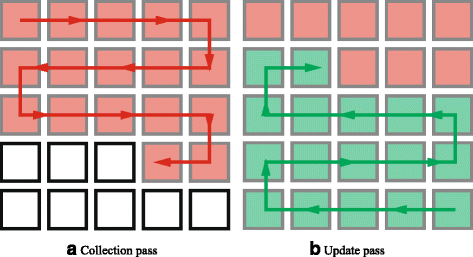

  

  Sequential update passes

• The update pass (Fig. 4 b) traverses the pixels in the update sequence (as in Fig. 3). In each step, it accumulates the contributions to the current pixel from all previous pixels that have already been updated (green), again in constant time. In addition, we add the contribution from all pixels that has not been updated to the current pixel (that is, the value of the corresponding red pixel from Fig. 4 a) to complete the update of the current pixel.

We first give a brief explanation of the constant time filtering process for accumulating the contributions to the expected energy and then show how the filter is employed in our two-pass algorithm. Gastal and Oliveira [8] showed that processing signals with infinite impulse response (IIR) filters can be performed using a summation of first-order recursive operations. In other words, a K-th order IIR filter that needs K feedback operations per pixel can be replaced with a summation of K first-order filters that need one feedback operation per pixel. For a two-dimensional signal f, two orthogonal 1D filters G in the horizontal direction and H in the vertical direction are used such that H∗G∗f corresponds to a 2D filtering of signal f.

First, the horizontal filtered result g _f =G∗f at pixel (y,x) is defined using a set of K first-order recursive operations,

$$\begin{array}{*{20}l} g^{+}_{f,s}(y,x,k) = a_{k}f(y,x) + b_{k}g^{+}_{f,s}(y,x-s,k), \end{array} $$

(7)

$$\begin{array}{*{20}l} g^{-}_{f,s}(y,x,k) = a_{k}b_{k}f(y,x+s) + b_{k}g^{-}_{f,s}(y,x+s,k), \end{array} $$

(8)

where $k=1\dots K, g^{+}_{f,s}(y,x,k)$ and $g^{-}_{f,s}(y,x,k)$ are the causal and anti-causal responses of the k-th first-order filter of signal f with complex coefficients a _k and b _k at pixel (y,x). Then,

$$ g_{f}(y,x) = \sum_{k=1}^{K} {{\text{REAL}}\left[g^{+}_{f,s}(y,x,k) + g^{-}_{f,s}(y,x,k)\right]} $$

(9)

is the response of the desired K-th order filter of signal f, which is computed by taking the real part of the summation of causal and anti-causal filter responses. The parameter s∈{1,−1} indicates the direction of first-order filters, where s=1 corresponds to a recursive operation from left to right in g ⁺ and right to left for g ⁻. Note that the choice of s does not influence the final filtered result g. Similar to the horizontal filtering, we define $h_{f}, h^{+}_{f,r}, h^{-}_{f,r}$ for vertical filtering, where the direction r∈{1,−1} manipulates the vertical index y. The 2D filtering of the signal f is then defined as

$$\begin{array}{*{20}l} H*G*f &= h_{g}(y,x) \\ & = \sum_{k=1}^{K} {{\text{REAL}}\left[h^{+}_{g,r}(y,x,k) + h^{-}_{g,r}(y,x,k)\right]}, \end{array} $$

(10)

which is the convolution of the two vertical and horizontal filters h and g. The reader is referred to Gastal and Oliveira [8] for more details about the filtering operations.

Next, we show that the 2D filter formulation in Eq. 10 can be computed recursively using the two-pass scheme as illustrated in Fig. 4 a, b. By expanding Eqs. 7 and 8, one can immediately see the relation between the causal and anti-causal filters, that is,

$$ g^{+}_{f,s}(y,x,k) = a_{k}f(y,x) + g^{-}_{f,-s}(y,x,k). $$

(11)

Using Eq. 11 once for h and once for g in Eq. 10, it is easily verified that the convolution result can be expressed by

$$\begin{array}{*{20}l} &h_{g}(y,x) = \\ &C^{-}_{f,r,s}(y,x) + \left(\sum_{k=1}^{K} {{\text{REAL}}[a_{k}]} \right)^{2}f(y,x) + C^{-}_{f,-r,-s}(y,x), \end{array} $$

(12)

where

$$\begin{array}{*{20}l} & C^{-}_{f,r,s}(y,x) \\ & = \sum_{k=1}^{K} {{\text{REAL}}\left[h^{-}_{g,r}(y,x,k) + a_{k}\sum_{k=1}^{K} {{\text{REAL}}\left[g^{-}_{f,s}(y,x,k)\right]} \right]}. \end{array} $$

(13)

The crucial insight from Eqs. 12 and 13 is that the 2D filtered output signal at pixel (y,x) is expressed as a sum of two contributions, $C^{-}_{f,r,s}(y,x)$ and $C^{-}_{f,-r,-s}(y,x)$, which represent the contributions from all pixels before (y,x) and all pixels after (y,x) in the update sequence. We compute $C^{-}_{f,-r,-s}(y,x)$ in the collection pass, and $C^{-}_{f,r,s}(y,x)$ in the update pass (Fig. 4 a, b). Note that the smoothness term between a pixel and itself is zero; hence, the expected smoothness energy for a variable is a sum over all other variables. Therefore, the middle term in Eq. 12 is zero.

All values in Eq. 12 can be computed with O(K) operations; therefore, the complexity to compute the expected energy is constant in the number of pixels and linear in the order K of the kernel function. Using this scheme, a Gaussian filter can be approximated perfectly (MSE<2.5×10⁻⁸) by using two recursive filters, that is K=2.

5.1.2 Efficient sequential update algorithm

Algorithm 2 shows the proposed sequential iteration of the mean-field approximation in a 2D fully connected grid with distribution Q using the update sequence from bottom right to top left (Fig. 4 b). First, the collection pass operates in reverse order (top left to bottom right) to compute and store the contributions to the expected energy from pixels in the sequence that have not been updated (Fig. 4 a).

In line 1, we compute the contribution to the expected energy from all previous variables on the current scanline using Eq. 8, illustrated in yellow in Fig. 5 a. In line 2, we compute Eq. 13, also illustrated in Fig. 5 a. We sum all contributions from previous variables in the horizontal (g ⁻, shown in yellow) and vertical directions (h ⁻, blue). This completes the collection step for the current pixel, and we store the result in a temporary buffer $\hat {Q}$. Next, lines 3–5 are needed to prepare for the next scanline. First, we compute g ⁺ using Eq. 7 in line 3, which we need to complete the horizontal filter g in line 4 (Eq. 9). In line 5, we accumulate the horizontal contributions g in the vertical direction (h ⁻) to be used in the next scanline. This is visualized in Fig. 5 b, where we apply the vertical anti-causal filter h ⁻ to the horizontally filtered contributions g.

Fig. 5

Visualization of the sequential update operations

Second, in the update pass, we now proceed in the update sequence order as in Fig. 4 b, with analogous computations to the previous pass. Here, we update the buffer $\hat {Q}$ by adding the contributions to the expected energies from the green (previously updated) half of the variables (line 7).

Note that in our algorithm we perform the update steps described so far for all hypotheses separately, but we omitted this in the notation for simplicity. To obtain the final expected energy of a pixel, we now need to perform the summation over all hypotheses (Eq. 4) in an inner loop (line 8). We also take into account the unary term here. The compatibility function of the hypotheses $w(d,l)=\exp (-|d-l|^{2}/{\sigma _{d}^{2}})$ corresponds to the third factor in Eq. 2. We then use the expected energy to update the distribution (line 9).

The proposed sequential update does not change the linear complexity of the algorithm in the number of pixels, however, it includes additional complex exponentials and multiplications for the IIR filtering (O(N M K) for N pixels, M hypothesis, and K-th order smoothness kernel). Although the sequential iteration is guaranteed to converge and minimize the KL-divergence, its result is biased with respect to the chosen update sequence due to the nature of the mean-field approximation (i.e., the result depends on the order in which variables are updated). To reduce this bias, in each iteration, we estimate the distribution over four sequences (top-to-bottom, bottom-to-up, left-to-right, and right-to-left) and update with the mixture of these distributions. Methods such as Jaakkola and Jordan [14] use the KL-divergence to optimally mix mean-field distributions; however, we found that simply averaging them is enough in our case.

5.2 Convergence results

We set up a toy experiment with synthetic data to compare the results of the parallel and sequential mean-field iteration. To have a baseline for our comparison, we also computed energies from Graph Cuts [2] with alpha-beta swaps. Further, in our experiment, we include the parallel update algorithm initialized with our SGM approach, as described in Section 4.3, to check the effect of our initialization. The other methods in this comparison do not include this initialization step. Similar to Kolmogorov [16], we compare the results from 50 randomly generated instances of unary data. Variables were distributed on a 39×29 grid with 16 hypotheses. The energy was defined over a fully connected graph with a smoothness term with Gaussian weights (σ=3) between them. We used a single CPU core (3.5 Hz) for all methods. Figure 6 shows the average energy (left) and KL-divergence (right) over the 50 random data instances for parallel, sequential, and SGM-initialized-parallel mean-field approximation implementations, in addition to Graph Cuts, as a function of computation time. The minimized energy indicates that with Gaussian weights on a fully connected graph, the mean-field approximation performs well compared to Graph Cuts. Both sequential and parallel mean-field approximations have linear time complexity in the number of variables and hypotheses; hence, they converge faster in contrast to Graph Cuts.

Fig. 6

Convergence comparison between parallel, sequential, and SGM-initialized parallel mean-field updates. We also include Graph Cuts minimization of our energy, which does not rely on the mean-field approximation. The KL-divergence cannot be evaluated for Graph Cuts since it only produces the MAP solution and not the full distribution

Without initialization, we observe that parallel updates (blue) converge to a higher energy and KL-divergence than the sequential approach (green). This confirms that sequential updates are more robust to local minima in the energy functional compared to the parallel approach. Initializing the distribution before parallel updates (red) using SGM (Section 4.3) leads to convergence to a lower energy and KL-divergence, closing the gap to the sequential approach. This is because SGM (as the first iteration of tree-reweighted message passing [6]) can find the global establishment of the variables to some extent. After the initialization, the parallel updates can refine the local configuration of the variables more independently. Note that at the beginning, the initialization increases the energy and KL-divergences sharply, because it tries to minimize a much simpler energy functional that does not necessarily have the same solution as our desired energy.

It is interesting to see that SGM-initialized parallel updates perform better than the sequential approach in terms of the KL-divergence (Fig. 6 (right)). This could be explained by the fact that, in contrast to the sequential approach, parallel updates do not suffer from directional bias. In practice, parallel updates can be implemented much more efficiently, for example, using GPU devices, since operations can be done for each pixel separately. Therefore, they are more attractive in practice. In the absence of a good initialization, however, the sequential update can be expected to obtain better results.

Finally, we compare sequential and parallel updates by computing end-to-end errors of the disparity maps from a subset of nine stereo images in the KITTI training dataset. In this comparison, we used the full pipeline proposed in Section 3 using a single core CPU implementation of the IIR filter. We also include results from an SGM-initialized version of the sequential method to see if initialization has a similar influence as in the parallel case. Figure 7 shows the percentage of pixels that have disparities differing by more than three pixels from their ground truth. These results agree with our previous experiments on energy and KL-divergence. Without initialization, sequential updates lead to better results than parallel ones. The SGM initialization improves both methods, and it closes the gap between them. The sequential update is about four times slower, however, since the distribution is computed with a mixture of four update sequences as described in the previous section.

Fig. 7

Comparing end-to-end results between sequential and parallel mean-field updates for a subset of KITTI stereo images

Fig. 8

Example results from the KITTI dataset. Top to bottom: left image, disparity map, and clamped disparity errors

6 Results and conclusions

As seen above, initialized parallel updates lead to best results in practice. Hence, in this section, we are reporting results and evaluations of this technique as described in Section 3 in more detail.

6.1 KITTI stereo evaluation

We first tested our CPU implementation without the temporal extension on the entire KITTI [9] dataset. We fixed parameters σ _s =4,σ _r =6,σ _d =4,λ=10⁹,γ=50λ, which we found by exhaustive search, and observed convergence after four iterations. Figure 8 illustrates our qualitative results from two scenes of the KITTI training dataset, where the first row shows the left input image, the middle row our final disparity map, and the last row the errors clamped to 5. In Table 1, we show the performance of each step of the proposed method in the KITTI training dataset. SGM initialization improves the quality about 30%. The proposed consistency term does not increase the computation time and further decreases the error by 10%. Table 2 summarizes the quantitative performance of our method on the KITTI test dataset. Our method obtains an average error of 3.32% for error threshold 3, and we currently rank number 8 on the list. Unlike other state-of-the-art methods, the proposed method does not have simplifying assumptions about the scene geometry such as piecewise planarity and does not assume prior knowledge on the data. Our CPU implementation compares to the rest in simplicity and scalability and still obtains state-of-the-art results.

Table 1 Performance of the each step of the proposed method

Table 2 The top 10 methods in KITTI benchmark

6.2 Stereo sequences

To measure the temporal coherence, we compared the flicker index (IESNA standard [4]) of the final disparity maps. This index is computed in a temporal window of five frames as the ratio of the time-averaged disparities and the disparities above that average, which indicates how much disparities deviate from their average value in a temporal window.

In Fig. 1, we compare the average flicker index of our GPU implementation with Richardt et al. [23] and Vogel et al. [28]. The plot on the right shows that we can significantly reduce the flicker index by enlarging the temporal smoothness kernel σ _t . In Table 3, we report the average computation times and flicker indices over five video sequences with resolutions from 417×360 to 960×540. Our GPU implementation requires less than 3 s per frame, and with σ _t =5, it produces significantly less temporal artifacts. Video results are available online for visual comparison.¹

Table 3 Flicker index

6.3 Conclusions

We have presented a robust method to compute disparity maps of stereo sequences in a single optimization. The optimization is solved efficiently using 4D filtering in pixel-disparity space. The proposed method ranks among the state of the art in challenging tests (KITTI) and produces less flicker artifacts in stereo videos.

We have developed a new and efficient filter-based optimization algorithm that performs sequential variable update in the mean-field approximation. This algorithm guarantees convergence along with a decrease of the KL-divergence in each iteration that is not available in previous filter-based mean-field approximation methods with parallel variable updates. In addition, our experiments showed that the new algorithm can perform well in comparison to Graph Cuts, a very well-established optimization method. We showed that with an intuitive initialization, the parallel scheme can perform as well as the sequential method. However, the right initialization might not be available all the time, in which case, the proposed sequential algorithm can be used instead.

7 Endnote

¹ http://www.cgg.unibe.ch/publications/temporally-consistent-disparity-maps

References

Bigdeli SA, Budweiser G, Zwicker M (2015) Temporally coherent disparity maps using CRFs with fast 4D filtering In: Pattern Recognition (ACPR), 2015 3rd IAPR Asian Conference on,301–305.. IEEE.
Boykov Y, Veksler O, Zabih R (2001) Fast approximate energy minimization via graph cuts. Pattern Anal Mach Intell IEEE Trans 23(11): 1222–1239.
Chakrabarti A, Xiong y, Gortler SJ, Zickler T (2015) Low-level vision by consensus in a spatial hierarchy of regions In: 2015 IEEE Conference on Computer Vision and Pattern Recognition (CVPR), 4009–4017.. IEEE.
DiLaura D, Houser K, Mistrick R, Steffy G (2000) The IESNA lighting handbook: reference & application,. 10edition. Illuminating Engineering Society of North America, New York.
Donatsch D, Bigdeli SA, Robert P, Zwicker M (2014) Hand-held 3D light field photography and applications. Visual Comput 30(6-8): 897–907.
Drorym A, Haubold C, Avidan S, Hamprecht FA (2014) Semi-global matching: a principled derivation in terms of message passing In: German Conference on Pattern Recognition, 43–53.. Springer.
Gastal ESL, Oliveira MM (2011) Domain transform for edge-aware image and video processing In: ACM Transactions on Graphics (TOG), 69.. ACM.
Gastal ESL, Oliveira MM (2015) High-Order Recursive Filtering of Non-Uniformly Sampled Signals for Image and Video Processing In: Computer Graphics Forum, 81–93.. Wiley Online Library.
Geiger A, Lenz P, Urtasun R (2012) Are we ready for autonomous driving? the kitti vision benchmark suite In: Computer Vision and Pattern Recognition (CVPR), 2012 IEEE Conference on, 3354–3361.. IEEE.
Güney F, Geiger A (2015) Displets: Resolving stereo ambiguities using object knowledge In: Proceedings of the IEEE Conference on Computer Vision and Pattern Recognition, 4165–4175.
Hermann S, Klette R (2012) Iterative semi-global matching for robust driver assistance systems In: Asian Conference on Computer Vision, 465–478.. Springer.
Hirschmuller H (2008) Stereo processing by semiglobal matching and mutual information. IEEE Trans. PAMI 30(2): 328–341.
Hosni A, Bleyer M, Gelautz M, Rhemann C (2009) Local stereo matching using geodesic support weights In: 2009 16th IEEE International Conference on Image Processing (ICIP), 2093–2096.. IEEE.
Jaakkola TS, Jordan MI (1998) Improving the mean field approximation via the use of mixture distributions. Learning in graphical models: 163–173. Springer.
Koller D, Friedman N (2009) Probabilistic Graphical Models: Principles and Techniques (Adaptive Computation and Machine Learning series), MIT press.
Kolmogorov V (2006) Convergent tree-reweighted message passing for energy minimization. Pattern Anal Mach Intell IEEE Trans 28(10): 1568–1583.
Krähenbühl P, Koltun V (2011) Efficient Inference in Fully Connected CRFs with Gaussian Edge Potentials In: Proc. NIPS, 109–117. http://papers.nips.cc/paper/4296-efficient-inference-in-fully-connected-crfs-with-gaussian-edge-potentials.pdf.
Lang M, Wang O, Aydin T, Smolic A, Gross MH (2012) Practical temporal consistency for image-based graphics applications. ACM Trans Graph 31(4): 34.
Mei X, Sun X, Zhou M, Jiao S, Wang H, Zhang X (2001) On building an accurate stereo matching system on graphics hardware In: Computer Vision Workshops (ICCV Workshops), 2011 IEEE International Conference on, 467–474.. IEEE.
Menze M, Geiger A (2015) Object scene flow for autonomous vehicles In: Proceedings of the IEEE Conference on Computer Vision and Pattern Recognition, 3061–3070.
Min D, Lu J, Do MN (2012) Depth video enhancement based on weighted mode filtering. IEEE Trans Imag Proc 21(3): 1176–1190.
Rhemann C, Hosni A, Bleyer M, Rother C, Gelautz M (2011) Fast cost-volume filtering for visual correspondence and beyond In: Computer Vision and Pattern Recognition (CVPR), 2011 IEEE Conference on, 3017–3024.. IEEE.
Richardt C, Orr D, Davies I, Criminisi A, Dodgson NA (2010) Real-time spatiotemporal stereo matching using the dual-cross-bilateral grid In: European Conference on Computer Vision, 510–523.. Springer.
Spangenberg R, Langner T, Rojas R (2013) Weighted semi-global matching and center-symmetric census transform for robust driver assistance In: International Conference on Computer Analysis of Images and Patterns, 34–41.. Springer.
Vineet V, Warrell J, Sturgess P, Torr P (2012) Improved Initialization and Gaussian Mixture Pairwise Terms for Dense Random Fields with Mean-field Inference. In: Bowden R, Collomosse J, Mikolajczyk K (eds)Proceedings of the British Machine Vision Conference, 73.1–73.11.. BMVA Press. doi:http://dx.doi.org/10.5244/C.26.73.
Vineet V, Warrell J, Torr PHS (2014) Filter-based mean-field inference for random fields with higher-order terms and product label-spaces. Int J Comput Vis 110(3): 290–307.
Vogel C, Roth S, Schindler K (2014) View-consistent 3D scene flow estimation over multiple frames In: European Conference on Computer Vision, 263–278.. Springer, ECCV.
Vogel C, Schindler K, Roth S (2015) 3D scene flow estimation with a piecewise rigid scene model. Int J Comput Vis 115(1): 1–28. Springer.
Yamaguchi K, McAllester D, Urtasun R (2013) Robust monocular epipolar flow estimation In: Proceedings of the IEEE Conference on Computer Vision and Pattern Recognition, 1862–1869.
Yamaguchi K, McAllester D, Urtasun R (2014) Efficient joint segmentation, occlusion labeling, stereo and flow estimation In: European Conference on Computer Vision, 756–771.. Springer.
Yu F, Gallup D (2014) 3d reconstruction from accidental motion In: Proceedings of the IEEE Conference on Computer Vision and Pattern Recognition, 3986–3993.. IEEE.
Zbontar J, LeCun Y (2015) Computing the stereo matching cost with a convolutional neural network In: Proceedings of the IEEE Conference on Computer Vision and Pattern Recognition, 1592–1599.
Zhang K, Fang Y, Min D, Sun L, Yang S, Yan S, Tian Q (2014) Cross-scale cost aggregation for stereo matching In: Proceedings of the IEEE Conference on Computer Vision and Pattern Recognition, 1590–1597.
Zhang K, Lu J, Lafruit G (2009) Cross-based local stereo matching using orthogonal integral images. Circ Syst Video Technol IEEE Trans 19(7): 1073–1079.
Acknowledgements
This research was supported by the Swiss Commission for Technology and Innovation (CTI) under project nr. 15592.1 PFES-ES.
Authors’ contributions
SAB performed the primary development and analysis for this work and the initial drafting of the manuscript. GB participated in the design and implementation of the proposed GPU pipeline. MZ coordinated SAB and GB to complete this work and played an essential role in editing the paper. All authors read and approved the final manuscript.
Competing interests
The authors declare that they have no competing interests.
Author information
Authors and Affiliations
Corresponding author
Rights and permissions
Open Access This article is distributed under the terms of the Creative Commons Attribution 4.0 International License (http://creativecommons.org/licenses/by/4.0/), which permits unrestricted use, distribution, and reproduction in any medium, provided you give appropriate credit to the original author(s) and the source, provide a link to the Creative Commons license, and indicate if changes were made.
About this article
Cite this article
Arjomand Bigdeli, S., Budweiser, G. & Zwicker, M. Temporally coherent disparity maps using CRFs with fast 4D filtering. IPSJ T Comput Vis Appl 8, 10 (2016). https://doi.org/10.1186/s41074-016-0011-2
Received:
Accepted:
Published:
DOI: https://doi.org/10.1186/s41074-016-0011-2